Introduction

Gaussian processes are becoming a popular machine learning method. GPs are non-parametric, which means that the actual number of "parameters" required scale (at least) linearly with the number of inputs being processed. In spite of this inconvenient feature, the flexibility and transparency of the modelling makes it an attractive method being intensively studied.

The main advantage of the GP inference is its nonparametric nature, i.e. we do not need a parametric model or function class that approximates the data but instead we give a non-parametric specification of the function class which is much richer.

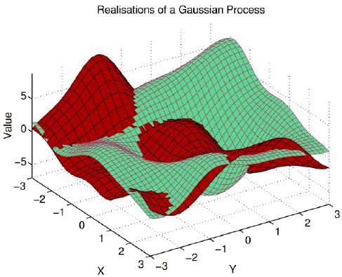
Choosing an RBF kernel function for the GP, one can compare the GP regression with regression using Radial basis functions (RBF). The difference is that for the RBF one has to specify the locations, in GP these are determined by the data (similarly to Support Vector Machines). The images below show realisations of prior GPs in one and two dimensions. Although there are local minima and maxima, no "centres" can be identified.

Too much freedom in choosing the interpolating function, or excessive richness of the function class might lead to overfitting - in GP inference this is avoided by the integration of the extra parameters. This is made possible by the framework of Bayesian inference.

Analytic tractability when using Gaussian Processes is restricted to normal noise or, equivalently, Gaussian likelihood function, for other likelihood models one has to use approximations.

Two successive approximations are employed in the GP inference presented here. A first one iteratively approximates the non-tractable posterior process with a GP (the origin of the online word in the title) and a second step which further simplifies the result by projecting it into a sparse support (the origin of the sparse term).

The result of the two approximation steps is a representation of the GP which relies only on a few selected input examples, the so-called Basis vectors. Since the approximation to the posterior is Gaussian, one can also optimise the hyper-parameters of the GP.

Inference in this framework is the inclusion of the input data (the training set) into the posterior process. This is done by assuming that we know the likelihood of the data and then by applying Bayes' rule one readily gets the posterior.

The picture below shows a one-dimensional example of the Bayesian inference, displaying the posterior mean function and possible samples from the posterior process (more in the Examples section).